Reference
Technical Annex#
The main report is written to be read without an engineering background. This annex serves readers who need the layer beneath it: how planners forecast future demand, characterize a load, decide through interconnection and transmission studies what to build, judge resource adequacy, model the system, analyze scenarios, assess reliability, trace distribution impacts, and fit the planning paradigms together. Each part cross-references the section it supports. Nothing here is required to follow the argument; all of it is required to act on it.
T.1 Data-center electrical architecture (supports the Primer and Section 4)#
Why this section exists. Every reliability argument in this report turns on what happens inside the facility between the utility feed and the processor, because that chain contains the protection devices that decide whether the load stays connected. A reader who treats a data center as a block of demand cannot evaluate a ride-through requirement, since the requirement applies to equipment inside the block. The architecture below is also what makes flexibility possible: the same uninterruptible supply that lets a facility disconnect cleanly lets it ride through a curtailment instruction, so Sections 4 and 6 describe opposite uses of one capability.
From the grid's point of view a data center presents not as a building full of computers but as a large, inverter-interfaced power-electronic load. Utility power arrives at medium-voltage switchgear at the facility point of interconnection, passes through uninterruptible power supply (UPS) systems that rectify AC to DC and invert it back — usually with battery storage on the DC bus — then flows through power distribution units to the racks, where server power supplies convert it once more. Every server therefore sits behind at least two stages of power-electronic conversion, so the facility presents to the grid as an inverter-dominated load with almost no rotating inertia to resist frequency change.
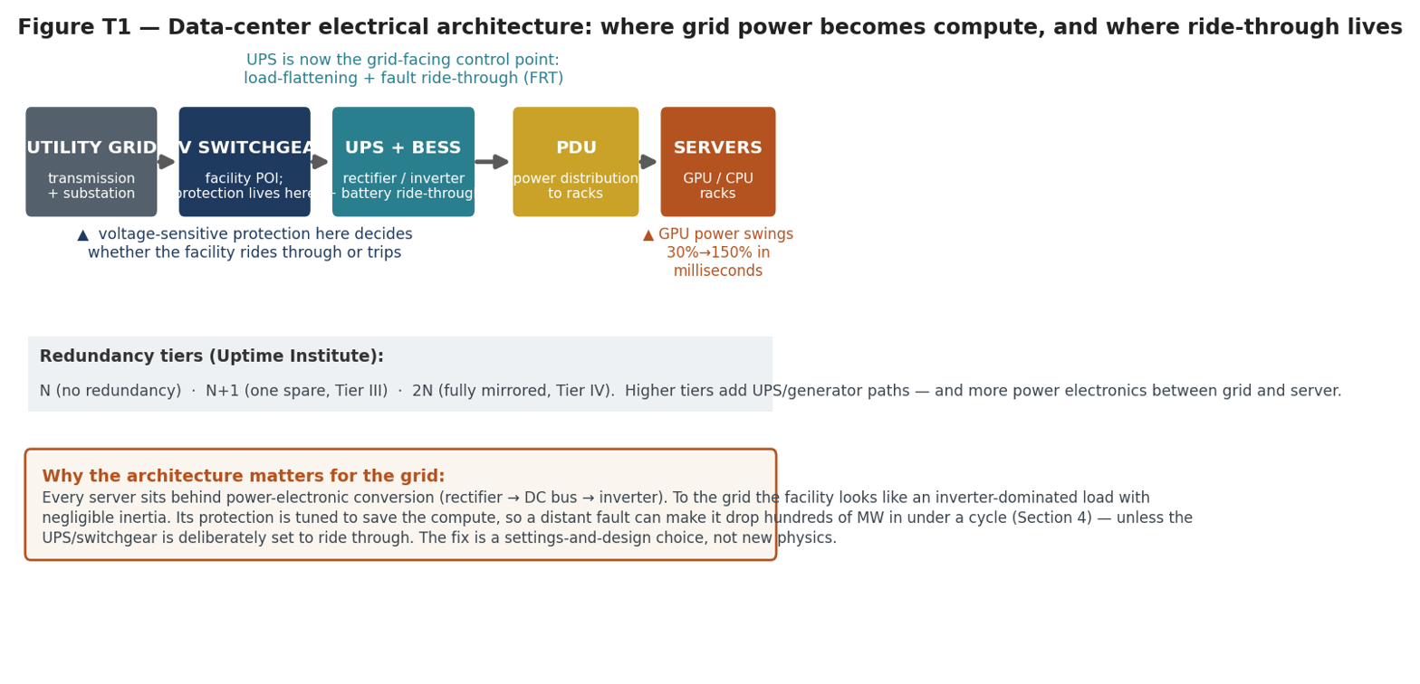
Figure T1 — The electrical chain from utility feed to processor. Four points in that chain determine how the facility behaves during a grid disturbance. Two were named when this report was written: the protection settings at the facility switchgear, and the uninterruptible supply that increasingly doubles as the grid-facing control point. Two more became load-bearing in 2025–26: the rack power shelf, which absorbs the fast transient, and the processor power controller, which carries the programmable ramp limit and power floor. The owner specifies all four, not the system operator, so facility behaviour during a fault stays largely invisible in planning models, and below the dashed line it is set by equipment design rather than by any tariff or standard. The reader should conclude that ride-through obligations and registration are the same problem approached from two directions (Section 4). Figure T8 draws the command hierarchy over this same chain.
Each stage of that chain removes information the grid would otherwise have. The medium-voltage switchgear sets the protective thresholds at which the whole site separates, and those settings are chosen by the owner rather than the operator. The transformer’s winding configuration determines whether an unbalanced fault reaches the equipment as an unbalanced sag or is partially tempered by a delta-wye arrangement — which is why NERC’s January 2026 reviews identified winding configuration as a root cause. The uninterruptible supply decides whether a disturbance produces a full transfer, a partial one, or none. By the time power reaches the rack, the facility’s response to a grid event has already been determined by three pieces of equipment the operator neither specifies nor sees.
The load beyond the rack is not uniform either, and the split matters for both reliability and flexibility. Roughly half to two-thirds of facility demand goes to IT load — servers, storage, networking — which the uninterruptible supply protects. The remainder is mechanical: chillers, computer-room air handlers, pumps and cooling towers. Mechanical plant is frequently not on the protected bus, because carrying it there would require far more battery and generator capacity. That asymmetry produces two consequences. Cooling can trip on a voltage sag while the IT load rides through, so a facility may shed in stages rather than at once. And thermal inertia in the cooling system is itself a flexibility resource — pre-cooling a hall before a curtailment window lets compute continue while mechanical load drops, which is the mechanism behind several of the demand-response arrangements in Section 6.
Two developments are changing the picture faster than the standards can follow. Rack power density has risen from roughly 5–10 kW in a conventional hall to 100 kW and beyond for accelerator racks, with 600 kW designs in prospect, which is what drives the shift to liquid cooling and concentrates a very large load into a small electrical footprint. And the battery in the uninterruptible supply is increasingly capable of acting as a grid resource rather than merely a buffer: the same hardware that lets a site island can, if the controls permit and the operator can see it, provide fast frequency response or hold load through a sag instead of dropping it. Whether that capability is used or merely present comes down to settings, which returns to the theme of Section 5 — capability the operator cannot see is capability the system cannot count.
Two architectural facts drive the reliability problem. First, redundancy: availability tiers (Uptime Institute's Tier I– IV, expressed electrically as N, N+1, or 2N) add parallel UPS and generator paths for resilience — which means more power electronics, and more protection logic tuned to protect the compute, sitting between the grid and the load. Second, the UPS has become the grid-facing control point. Traditional “UPS-last” designs treated backup power as a downstream facilities component; modern AI-oriented designs place a medium-voltage UPS with battery storage as a high-bandwidth control point that can, in principle, flatten load and provide fault ride-through. That same equipment, set conservatively, also disconnects the facility in under a cycle during a distant fault (Section 4). The fix for uncommanded tripping turns largely on UPS design and protection settings — a configuration choice, not new hardware physics.
A second grid-facing control point has since appeared below the UPS, inside the rack. NVIDIA's GB300 NVL72 power shelves carry electrolytic capacitors that charge while GPU demand is low and discharge while it is high — about 65 joules per GPU, occupying roughly half the volume of the shelf, co-designed with LITEON — under a charge-management controller that runs the smoothing at rack level. Tested against a GB200 rack on the same training job, the vendor reports the grid-facing peak reduced by about 30% at identical GPU output, and says the feature is being extended to GB200 systems. Two consequences follow for the grid. The rack, not the facility, now absorbs the fastest transients, so the load the UPS sees is already partly flattened and the facility need not be provisioned for maximum instantaneous draw. And the storage is deliberately one-directional: it shapes the profile presented to the grid and returns no energy to the utility, so it is not a resource in any market sense and should not be counted as one. Vendor documentation, primary; the durability of electrolytic capacitors in high-temperature service is a reported caveat.
The mitigation is real and it is bounded, and the bound is what a standard has to be written against. On the published figure of 65 joules per GPU an NVL72 rack stores about 4.7 kJ. Measured against the swing rather than the whole load — roughly 40 kW, on the vendor's own 30% figure and a rack rated near 135 kW — that is on the order of 115 milliseconds of coverage, and less in service, since a capacitor bank discharged to 70% of rated voltage yields about half its stored energy. Half-cycles in the 0.2 to 3 Hz emission band run from 167 milliseconds to two and a half seconds. The buffer therefore cannot span a single half-cycle even at the fastest end of the band, which is why the joint paper recommends GPU-level smoothing and rack storage together rather than either alone. At the GPU layer the same work reports a minimum power floor that cannot be set above 90% of thermal design power, leaving at least a fifth of TDP as residual dynamic range at an energy cost near 10.5%. A utility specification demanding a tighter dynamic range than that is not met by this generation of hardware. Rack energy and coverage derived here from the published per-GPU figure and rack rating; the discharge-depth allowance is an engineering estimate, not a vendor figure.
That bound is generational, not permanent, and the report should say so rather than rest an argument on it. The announced 800 VDC architecture moves power conversion out of the rack for megawatt-class systems from 2027, and the vendor states that the Vera Rubin NVL144 design carries on the order of twenty times the energy storage of the current generation. If that holds, coverage moves from roughly a tenth of a second toward seconds — inside the emission band rather than below it. The conclusion for §4 is not that the hardware will or will not solve this. It is that equipment capability is moving faster than the standards drafting it, so a standard written against measured 2024–26 behaviour, or against any named platform, dates immediately. 800 VDC timing and the storage multiple are vendor announcements; neither has been demonstrated in service.
Planning implication. Because the behaviour that matters is set below the meter and specified by the owner, the binding constraint becomes visibility rather than cost. The operator cannot require, credit, or even verify what it cannot see, so the architecture described here turns into an operations and registration problem the moment the facility energises (Sections 4 and 5).
T.2 Industrial load characteristics: why computational load differs in kind (supports Sections 4 and 6)#
Why this section exists. Planning practice rests on a century of observed load behaviour — diversity, weather sensitivity, predictable ramps — and each of those regularities is an empirical fact about the load mix rather than a law. This section sets out which of them computational load breaks and which it preserves, because the answer determines which planning tools remain valid. Where the load resembles conventional industrial demand, existing methods transfer; where its coincidence factor approaches one and its output is insensitive to weather, they do not, and the forecasting and adequacy problems in T.5 and T.6 follow directly from that difference.
Large industrial loads are not new; aluminum smelters, steel mills, and chlor-alkali plants have drawn hundreds of megawatts for decades. The novelty lies in the electrical signature. Traditional heavy industry draws a relatively steady load with a high load factor and, crucially, often tolerates interruption and changes slowly. AI training clusters invert every one of those properties. Thousands of GPUs ramp in lockstep at mini-batch boundaries, producing quasi-periodic, multi-megawatt power swings over seconds — and instantaneous swings from roughly 30% to 150% of nominal within milliseconds at the rack level. Aggregated to gigawatt scale, published estimates put the resulting system-level ramp rates above 1,000 MW per second, and field measurements have documented forced oscillations (a 14.7 Hz mode in one study) that can couple with weakly damped grid modes. The contrast is worth making precise, because it explains why existing planning methods become less accurate:
| Characteristic | Traditional heavy industry | AI training data center | Crypto mining |
|---|---|---|---|
| Load factor | High, steady | High but volatile (bursty) | High; can idle instantly |
| Ramp behavior | Slow, gradual | Multi-MW swings in seconds; >1,000 MW/s aggregated | Near-instant on/off |
| Inertia contribution | Rotating motors add some | Negligible (inverter-fed) | Negligible |
| Fault behavior | Rides through; motor loads | Voltage-sensitive trip via UPS/protection | Trips or self-curtails |
| Flexibility | Limited; process-bound | Real but SLA- and checkpointconstrained | High (economics-driven) |
| Power quality | Harmonics from drives | Harmonics + fast transients + oscillations | Harmonics; switching |
Table T2A — Computational load against the industrial load the system was built around. The rows that matter are ramp rate and controllability: a smelter is large but slow and contractually interruptible, while a training cluster is large, fast, and governed by a scheduler the operator cannot see.
Sources: NERC; ERCOT; EPRI; and the peer-reviewed and preprint literature listed in the Technical Annex references.
The practical implication: a planner who models an AI campus with the assumptions appropriate to a steel mill will understate both its instability risk (Section 4) and, paradoxically, its flexibility potential (Section 6). Computational load proves simultaneously more dangerous and more controllable than the industrial load it superficially resembles.
Three properties deserve separate statement, because each breaks a different planning assumption. Coincidence. Aggregate load has always been smaller than the sum of individual peaks, because customers peak at different times, and the whole apparatus of diversity factors rests on that. A fleet of facilities running near maximum around the clock has a coincidence factor approaching one, so its contribution to system peak approaches its full connected load — and, being built to common reference designs with common protection settings, it also responds to a disturbance in unison. Diversity fails on both the demand side and the fault-response side at once.
Weather insensitivity. Conventional load forecasting reduces largely to weather modelling: heating and cooling drive the peaks, and the relationship between temperature and demand forms the strongest signal in the data. Computational load barely responds to weather on the IT side, though its cooling load does. The consequence is not that it is easier to forecast but that the established method does not apply — and, more seriously, that it adds to demand in extreme temperatures without the offsetting behaviour that other load classes show, arriving at full strength in precisely the hours when the supply side is most degraded (T.6).
Ramp rate. A steel mill’s arc furnace cycles on a schedule an operator can anticipate. A training cluster changes power by a large fraction of its rating in seconds when a job starts, checkpoints or fails, and synchronised workloads across thousands of accelerators make those swings coherent rather than averaging out. Reported behaviour runs to tens of percent of nominal rack power within tens of milliseconds, aggregating to hundreds of megawatts per second at campus scale. No North American jurisdiction presently imposes a generally applicable ramp-rate limit on an individual large computational load, though individual service agreements may contain one, which is the gap Section 4 identifies; the market procures the load-following resource that must absorb the swing without anyone specifying how large the swing may be.
T.3 Interconnection and transmission studies: can the existing grid take the load? (supports Sections 1 and 5)#
Why this section exists, and how the studies are used. An interconnection study is the gate through which every project in Section 1’s queue must pass, and its sequence explains both the duration of the queue and where it can be shortened. The studies run in a fixed order because each depends on the one before: a feasibility screen establishes whether an obvious constraint exists, a system impact study quantifies the constraint and identifies upgrades, and a facilities study prices and schedules them. Each stage assumes a set of prior projects already connected, so a withdrawal upstream forces restudy downstream — the mechanism behind cluster processing and the readiness deposits that Order No. 2023 introduced on the generation side and that large-load reform is now copying.
For the reader, the operative point is what these studies do not decide. They establish whether the network can carry the load and what it costs to make it do so. They do not establish whether enough generation exists to serve the load over a year (T.6), whether the load will behave acceptably during a disturbance (T.4 and T.8), or whether anyone should bear the cost (Section 3). A project can clear every study and still present each of those three problems, which is the structural reason this report treats interconnection and adequacy as separate sections rather than stages of one process.
When a large load applies to connect, the operator must answer a deceptively simple question: can the existing transmission system serve it reliably, and if not, what must be built? A staged process governed by NERC's transmission planning standard TPL-001 (currently TPL-001-5.1) answers it, requiring the system to withstand a defined spectrum of contingencies without cascading or uncontrolled load loss. The studies run in a fairly consistent order, each a gate the project must pass:
- Feasibility / screening. A first-pass look at whether the point of interconnection has obvious capacity, and at rough upgrade scope. In batch regimes (ERCOT's Batch Zero) the operator pools and ranks requests against shared transmission limits rather than studying them one at a time.
- Steady-state power-flow (load-flow) study. Solves the network under normal and contingency conditions to check for thermal overloads on lines and transformers and for voltage violations (typically outside 0.95–1.05 pu). This study most often produces the upgrade list.
- Short-circuit (fault-duty) study. Compares fault current before and after the load (and any associated generation) against breaker interrupting ratings per TPL-001-5.1; if the addition pushes a bus over its breaker rating, equipment must be replaced.
- Transient-stability (RMS dynamic) study. Exercises the load's dynamic model against the network to evaluate frequency response, voltage recovery, ramping, energization inrush, load tripping/reconnection, and fault ride-through against the operator's disturbance-performance requirements.
- EMT screen at weak-grid points. Where local system strength runs low (screened by short-circuit ratio and its weighted/composite variants and by critical clearing time), a full-waveform electromagnetic-transient study becomes mandatory to catch control-interaction instabilities that RMS tools miss. SPP's HILL process makes this gate explicit. What comes out the other end is an upgrade list and its cost. Typical remedies escalate in expense and lead time: reconductoring an existing line with higher-capacity conductor, adding or upgrading transformers, installing reactive support (capacitor banks, STATCOMs, or SVCs) to hold voltage, and — the expensive, slow end — building new lines or substations. The contingency framework is the heart of the analysis: planners test the loss of single elements (N-1) and combinations (N-1-1), sizing the system against the largest credible loss. The large-load era breaks two assumptions inside it. First, load historically behaved as a passive, roughly predictable quantity — not a contingency that can vanish in a cycle; NERC's 2026 guidance now asks planners to treat the sudden loss of a clustered large load as a studied contingency comparable to losing a large generator (BAL-002's Most Severe Single Contingency). Second, because data centers cluster, the local grid can be too weak for stable inverter-dominated operation — the precise condition the EMT screen exists to catch. Who pays for the resulting upgrades is the cost-allocation fight of Section 3; whether the study even sees the failure mode is the modeling problem of T.4.
Two features of this sequence explain most of the delay that Section 1 describes. Each study is performed against a base case that assumes a specific set of prior projects already connected, so a withdrawal upstream changes the answer downstream and forces restudy — the restudy cascade that serial queues produce and that cluster processing exists to prevent. And the studies are sequential by necessity rather than by convention: a stability study cannot be run before the power flow that defines its operating point, and an EMT screen is meaningless until short-circuit analysis has established where grid strength is low. Reforms that shorten the queue therefore work by reducing the number of times the sequence is run, not by running it faster.
What the studies produce is a list of network upgrades with costs and construction lead times, and that output is the hinge between the engineering and everything else in this report. The upgrade list determines the interconnection cost that Section 3 argues about allocating. The construction lead times — four years for a large transformer, longer for a new line — set the energisation date that Section 2 finds the load outrunning. And the studies establish which network conditions bind, which is what makes conditional and curtailable service possible at all: a load willing to reduce when a constraint binds can often be served without the upgrade — the structure of SPP’s CHILLS and of European flexible connection agreements (Section 6).
T.4 Power-system modeling: the tool decides what the study can see (supports Section 4)#
A study can only match its load model, and the record here weighs heavily against the legacy practice. For decades, load in stability studies was represented statically — as a fixed or voltage-proportional P–Q injection (the ZIP or constantpower model). A static model cannot represent a load that disconnects itself during a voltage sag, so a study built on one will report that a facility rides through a fault it would in reality trip on. That gap amounts to more than rounding: it separates seeing the dominant failure mode from missing it.
Before the load model itself, it is worth setting out what each class of study is for, because the terms recur throughout this report and the distinctions decide which questions a given analysis can answer. The four study types below run in sequence during an interconnection review, and the three load models beneath them determine what each of those studies sees.
| Model or tool | What it represents | What it is used for | What it cannot see |
|---|---|---|---|
| Power flow (steady state) | The network at one instant: voltages, angles, and flows for a fixed dispatch and load. | The first screen in any interconnection study — whether adding the load overloads a line or drives a bus outside its voltage band, under normal and contingency conditions. | Time. It has no dynamics, so it cannot show what happens during or after a fault, only the condition before and the condition after. |
| Short-circuit study | Fault current magnitude and distribution for faults at each bus. | Sizing breakers and coordinating protection; establishing whether existing equipment can interrupt the available fault current once new sources are added. | Load behaviour. It answers what the network delivers into a fault, not how connected equipment responds to one. |
| Positive-sequence dynamic (RMS) simulation | Machine and control dynamics at fundamental frequency over seconds to tens of seconds. | The standard transient stability study: whether generators stay synchronised and voltage and frequency recover after a contingency. | Waveform-level behaviour. It approximates power-electronic control loops and current limits, which is why it is unreliable for inverter-dominated interfaces. |
| Electromagnetic transient (EMT) simulation, PSCAD class | Full instantaneous waveforms, including converter switching, control loops and protection logic, at microsecond resolution. | Required where power-electronic content is high or grid strength is low — and, under NERC’s May 2026 alert, at large-load points of interconnection. It is the only class of study that reproduces the trip behaviour in Section 4. | Scale. It is computationally expensive and run on a reduced network, so it answers local questions rather than system-wide ones. |
| Static load model (ZIP or constant power) | Load as a fixed or voltage-proportional real and reactive power draw. | Legacy practice in stability studies, adequate while load was predominantly motors and resistive heating. | Self-disconnection. It cannot represent a load that trips on a voltage sag, so a study using it reports ride-through where the facility would in fact leave. |
| WECC composite load model (CMPLDW) | A mix of motor classes, static load, electronic load and distributed generation behind a representative feeder. | The industry workhorse for distribution-connected load in stability studies. | Computational load. Built to capture motor-driven feeders; NERC has stated explicitly that it does not represent the parameters that make large data-center load risky. |
| PERC1 | Purpose-built computational load: voltage-sensitive trip threshold and duration, reconnection voltage and delay, IT versus non-IT load fraction, and UPS transfer logic. | Required by NERC’s Level 3 alert for planners studying these facilities, or a model of equivalent or better capability. It is the precondition for enforcing a ride-through standard — an obligation cannot be required if it cannot first be simulated. | Facility-specific settings it is not given. The model is only as good as the parameters an operator can compel the owner to provide (Section 4). |
| PERC2 and the Data Center Load Modeling Technical Reference | Successor specification and the accompanying parameter guidance. | In development; intended to standardise how these facilities are represented across regions rather than leaving each planner to its own assumptions. | Not yet issued at the date of this report. |
Table T4A — What each model is for. The final column is the operative one: every model in this table abstracts the system to make a specific question tractable, and each stays silent on questions outside that purpose. The failures described in Section 4 were not modelling errors so much as the use of a model outside the range of questions it was built to answer.
Sources: NERC Level 3 Essential Action Alert (May 2026) and accompanying reliability guideline; WECC composite load model documentation.
Two practical points follow. The models accumulate rather than replace one another: a planner runs power flow to find the binding constraints, short-circuit to check the equipment can clear a fault there, positive-sequence dynamics to confirm the system recovers, and EMT only at the interfaces where the previous step cannot be trusted. And the load model feeds the last two rather than standing as a study in its own right — which is why substituting PERC1 for a static representation changes the answer without changing the study, and why the modelling reform is the precondition for every reliability requirement that follows it.
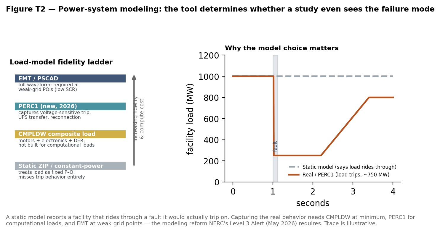
Figure T2 — The fidelity ladder and why it matters. The same disturbance produces opposite conclusions depending on the load model: a static model shows ride-through; a computational-load model shows the trip that actually happens. The same ladder runs through the simulation method itself: a static representation, then positive-sequence (RMS) dynamics, three-phase RMS, full electromagnetic-transient (EMT) simulation, and finally hardware-in-the-loop testing — each rung resolving faster phenomena at higher computational cost, and each warranted only where the rung below it cannot answer the question.
The industry's workhorse dynamic model, the WECC composite load model (CMPLDW), marked a large step up — representing a mix of motor types, static load, power electronics, and distributed resources — but its developers built it to capture motor-driven distribution feeders, not gigawatt computational loads, and NERC has been explicit that it does not capture the parameters that make these loads risky. In response came a new model, PERC1, purpose-built to represent the voltage-sensitive trip threshold (the voltage and duration at which the load disconnects), the reconnection voltage and time delay, the split between IT and non-IT load fraction, and the UPS transfer logic. NERC's Level 3 Alert (May 2026) requires planners to use PERC1 or a model with equivalent-or-better capability, and to add full-waveform EMT (PSCAD-class) modeling at weak-grid interconnections or where power-electronic content is high. A Data Center Load Modeling Technical Reference and a PERC2 specification are following. The modeling reform sets, in a real sense, the precondition for every other reliability fix: you cannot require ride-through performance you cannot first simulate. Two further modeling frontiers matter for planning. First, inverter-based representation: because the facility interfaces the grid through power electronics with negligible inertia, planners must model it the way they now model inverter-based generation — with explicit control loops, current limits, and fault-current behavior that positive-sequence tools approximate poorly, which is why EMT is increasingly mandatory at the point of interconnection. Second, flexibility representation: if a large load is to be credited as curtailable (Section 6) or accredited for adequacy (T.6), the model must separate firm from flexible load components, represent behind-the-meter generation and storage, and reflect operating windows such as AI-training schedules. A model that carries a flexible gigawatt as a firm subtraction from demand will misstate both the reliability risk and the reserve value — the reason NERC's guideline asks explicitly for firm-versus-flexible decomposition.
How the study is actually performed. The preceding pages say what each model represents and why the load model decides the answer. They do not say how an engineer chooses between them, parameterises them, or knows when a study has stopped being trustworthy. Those judgments carry most of the practical risk in this subject, because a study that is run correctly against the wrong assumption returns a clean result and a false assurance. What follows is the working guidance, stated as practice rather than as requirement — the mandatory elements appear in the NERC Level 3 Alert described above.
- When RMS is sufficient. Positive-sequence RMS (phasor) simulation assumes a balanced system at fundamental frequency and represents the network by its impedance, a good approximation for phenomena slower than roughly five to ten hertz. That covers most of what a planner does: angular and voltage stability against normally cleared faults, governor and exciter response, inter-area oscillations, and the large screening runs across many contingencies that no EMT tool could complete in the time available. RMS remains the right first instrument for a large load whose behaviour is well characterised and whose trip settings are represented in the load model. It stops being sufficient at the point where the answer depends on what happens inside the cycle.
- When EMT is required. Four conditions, any one of which is sufficient. A weak interconnection, conventionally a short-circuit ratio below about three, where the converter's control loops and the network interact rather than acting in sequence. High power-electronic content at the point of interconnection — inverter-based generation, storage, HVDC, or the rectifier front end of the load itself — where control interactions and sub-synchronous oscillations live above the phasor model's ceiling. Any question whose answer depends on sub-cycle behaviour: fault ride-through at the equipment's own trip threshold, protection coordination, unbalanced faults, harmonic interaction, or the transfer of a UPS. And any case where the RMS study returns a marginal result, since marginal in phasor terms provides no evidence of margin. The Level 3 Alert makes the first two mandatory rather than discretionary at weak-grid interfaces and where power-electronic content is high.
- Which model, and how to parameterise it. For conventional motor-driven feeders the composite load model remains the right tool, parameterised from feeder composition — the motor fractions by class, the static and power-electronic fractions, the distributed-resource share, and an equivalent feeder impedance — drawn from end-use data rather than from library defaults, which are regional averages and belong to someone else's system. Where computational load is material the composite model is the wrong instrument at any parameterisation, because the quantities that decide the outcome sit outside it: NERC's Level 3 Alert directs planners to PERC1 or an equivalent, whose four governing parameters — the voltage and duration at which the load disconnects, the voltage and delay at which it returns, the IT to non-IT split, and the UPS transfer logic — can only come from the customer. That is the practical significance of the registration and data-provision requirements in Section 4: without them the model has no inputs, and the study reverts to an assumption.
- Validating an inverter or UPS model. Validation means benchmarking the model against measurement, not confirming that it runs. The practical sequence is: a flat start, confirming the model initialises and holds steady with no disturbance applied — a model that drifts here will produce plausible nonsense later; response tests against voltage and frequency steps and against a fault-and-recovery profile, compared with factory or commissioning records; and, where measurement exists, replay of a recorded system event through the model, with the discrepancy characterised rather than tuned away. For power-electronic equipment the RMS and EMT representations must also be benchmarked against each other on a common disturbance: where they disagree, the EMT result governs and the RMS model needs the work. Vendor-supplied models should be treated as unvalidated until the settings in them match the settings commissioned on site, which is the point at which most of the disagreement is found.
- What invalidates a study. Six assumptions do most of the damage, and all of them are defaults rather than decisions. A static or ZIP load representation, which cannot trip and therefore cannot reproduce the event the study is meant to examine. A load model with no trip logic or no reconnection logic, which converts an uncommanded loss of demand into a smooth voltage recovery. Aggregation at the transmission bus, which averages away the distribution-level behaviour that decides whether the load rides through. Positive-sequence representation of an unbalanced event, which understates the phase-to-ground voltage the equipment actually sees. Generic inverter models left at library defaults, which encode a manufacturer's example rather than the installed settings. And a single peak-load case, which is the wrong condition for a computational campus whose worst hour for the system may be a light-load night. A study carrying any of these is not conservative; it stays silent on the failure mode.
Planning implication. Because planners can evaluate only what their models represent, an inappropriate study method understates both the upgrade list and the operational risk — and does so silently, returning a clean result for the wrong question. The modelling reform of Section 4 therefore does not merely refine the analysis; it makes the reliability requirements that depend on it possible at all.
Sources: NERC Level 3 Essential Action Alert (May 2026) and accompanying reliability guideline; WECC composite load model documentation and model validation guidance; NERC modelling notifications and inverter-based resource performance guidelines; IEEE 2800 model-validation provisions. Stated as engineering practice, not as a filed position.
T.5 Load forecasting: methods, load types, and uncertainty (supports Section 1)#
Why this section exists, and what the methods are for. Every number in Sections 1 through 3 rests on a forecast, and forecasts of large load are produced by a different method from the econometric extrapolation that served a stable system. The conventional approach regresses historical consumption on weather and economic drivers, which works when next year’s load is a modest perturbation of this year’s. It fails when a single customer can add several percent to a zone, because the historical series contains no analogue. The replacement is a bottom-up, project-based method: enumerate the specific requests, assign each a probability of proceeding, apply a load factor and ramp schedule, and sum. The probability weighting separates a forecast from a queue total, and the assumptions listed below explain how two forecasters using the same method arrive at answers differing by a factor of three.
Section 1 introduced the three forecasting families (econometric top-down, bottom-up project-weighting, and probabilistic scenario). This part adds the two things a forecaster must get right beneath the method: how different large loads are characterized, and how uncertainty is carried through. Characterizing the load matters because “data center” is not one thing. Each type presents a different shape to the grid, and a forecast that lumps them together will misjudge both peak and flexibility:
- AI training clusters. Very high load factor, run flat-out around the clock, but with second-scale synchronized swings; near-unity coincidence with system peak. Some scheduling flexibility, constrained by checkpoint overhead.
- AI inference / cloud. High, steadier load tied to user demand; more diurnal shape; tighter service-level agreements limit curtailment.
- Traditional colocation. Moderate, diverse tenant mix; the closest to legacy commercial load; more predictable.
- Cryptocurrency mining. High load factor but highly price-responsive — can idle in seconds when power prices spike or the grid tightens, making it the most flexible of these load classes by nature.
Beneath the method sit five assumptions that move the answer as much as the request-weighting does. A careful reader should interrogate each before trusting any large-load forecast. Coincidence and diversity: AI training carries a coincidence factor near one, so assuming legacy diversity understates its peak contribution. Load factor and ramp schedule: how fast a campus reaches full draw, and how flat it then runs. Developers supply both through attestation letters, such as ERCOT's “Officer Letter Loads,” and the forecaster must decide how far to trust them. Spatial allocation: because loads cluster, a forecast reasonable statewide can badly understate one zone — PJM adjusted 14 of 15 zones in 2026. Weather and economic normalization: the econometric base rests on weather and macro inputs such as Moody's Analytics data. Probability weighting: feasibility-stage against contracted load, among the largest swing factors and the least standardized of the five. Uncertainty suffers frequent mishandling. Because these dials are set independently and rarely disclosed together, point forecasts across the industry diverge by a factor of three. The mature response is not a single number but a distribution: a reference case bracketed by high- and low-growth scenarios, ideally probabilistically weighted, with the spread itself reported as information. NERC's March 2026 gaps assessment put it plainly — existing load-forecasting methods may be insufficient for loads that bid into multiple areas at once, overstating expected demand. A forecast measures nothing; it stacks assumptions. Reading one honestly means asking which dials were turned, how far, and how wide the resulting band is. That posture leads directly into scenario analysis (T.7).
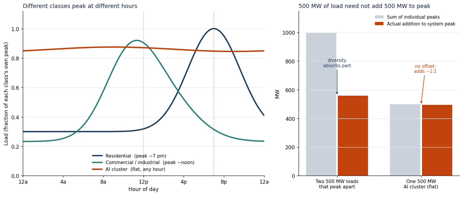
Figure T7 — Coincident versus non-coincident peak. Residential load peaks in the evening and commercial-industrial load near midday, so their combined peak falls below the sum of the two — diversity absorbs part of it. A flat, high-load-factor AI cluster has no such offset: it sits near full value in every hour, including the system peak, so it adds to peak almost one-for-one. Shapes are schematic, each normalised to its own peak.
T.6 Resource adequacy planning: will there be enough generation and reserves? (supports Section 2)#
Interconnection studies (T.3) ask whether the wires can carry the load. Resource adequacy planning asks a different question: across a whole year of weather, outages, and demand variation, will there be enough accredited generation and reserves to keep the lights on to an agreed standard of reliability? The answer is expressed in a small set of probabilistic metrics that a reader of any RTO assessment will encounter.
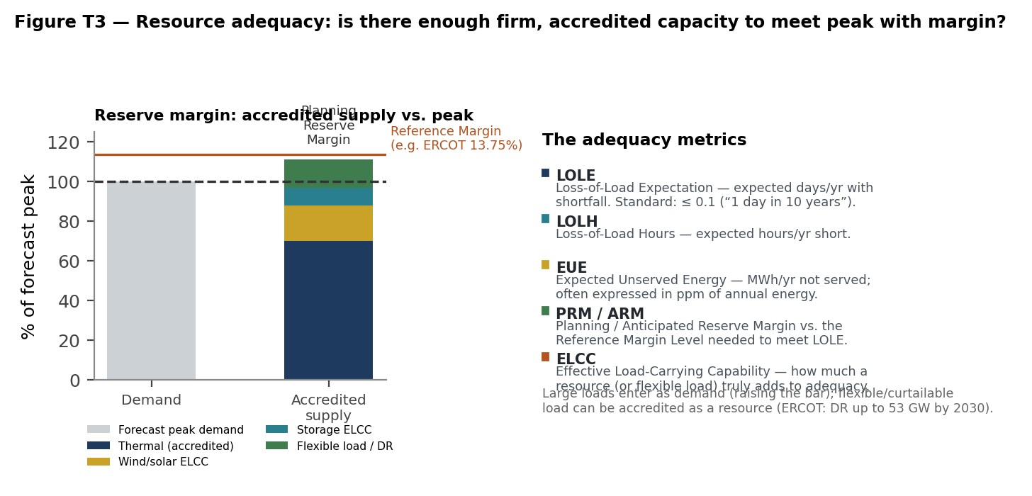
Figure T3 — The two halves of adequacy: is accredited supply above peak with adequate margin (left), and do the probabilistic metrics stay within their thresholds (right)? Large loads raise the bar; flexible loads can be accredited to help meet it.
The reliability standard is conventionally a loss-of-load expectation (LOLE) no worse than 0.1 days per year — the familiar “one day in ten years.” Around it sit companion metrics: loss-of-load hours (LOLH), expected unserved energy (EUE, often expressed in parts-per-million of annual energy), and the planning or anticipated reserve margin (PRM/ARM) compared against the reference margin level needed to satisfy LOLE. These are computed with probabilistic assessments (ProbA) — Monte Carlo simulations over many combinations of weather years, loadforecast uncertainty, and generator forced outages (SERC, for instance, runs thousands of simulations per hour across four decades of weather). The 2026 assessments indicate the strain: PJM's anticipated reserve margin has fallen sharply, and NERC places several regions at elevated or high risk beginning around 2028–2029. Large loads change the calculation in two directions. As demand, they raise the bar — more accredited capacity is needed to hold the same LOLE. Genuine flexibility, however, lets them earn accreditation as a resource: ERCOT's 2025 assessment credits demand response rising toward 53 GW by 2030 and notes that because new large loads can be curtailed during emergencies, their rapid growth has substantially less effect on reserve margins than a firm forecast would imply. The accreditation method matters enormously — ERCOT's switch from historical peakcapacity factors to probabilistically-derived effective load-carrying capability (ELCC) for wind and solar materially cut their credited contribution. The frontier question, now in the literature, asks how to accredit co-located load-plus-generation-plus-storage systems, where naive approaches (summing individual ELCCs) produce large errors. Getting accreditation right determines whether a flexible gigawatt counts as a problem or part of the solution.
The distinction between the two questions is worth stating carefully, because they are routinely conflated in public argument. An interconnection study is deterministic and local: it asks whether a specified network, under a specified condition, holds. Adequacy planning is probabilistic and system-wide: it asks how often, across thousands of possible years, supply falls short anywhere. A system can pass every interconnection study and still be inadequate, and it can be adequate in aggregate while a particular corner of the network cannot be served. The two failure modes have different remedies — wires for the first, capacity or demand reduction for the second — the reason Sections 1 and 2 treat them separately.
| Metric | What it measures | Conventional threshold | What it misses |
|---|---|---|---|
| LOLE — loss-of-load expectation | The expected number of days per year on which available supply falls short of demand at any point in the day. | 0.1 days per year, the familiar “one day in ten years.” | Duration and depth. A one-hour shortfall of 50 MW and a twelve-hour shortfall of 5 GW each count as one event. |
| LOLH — loss-of-load hours | The expected number of hours per year of shortfall. | No universal standard; used alongside LOLE to expose duration. | Magnitude. It counts hours, not megawatts unserved. |
| EUE — expected unserved energy | Expected megawatt-hours of demand that cannot be served, often normalised as parts per million of annual energy. | No universal standard; the metric most sensitive to depth. | Timing and concentration. The same annual EUE may fall in one severe week or spread thinly. |
| PRM and ARM — planning and anticipated reserve margin | Accredited capacity above forecast peak, as a percentage. | Compared against a reference margin level set so the system meets 0.1 LOLE. | Everything the accreditation step already decided. A margin is only as meaningful as the ELCC values behind it (Table 2A). |
| ELCC — effective load carrying capability | How much perfectly firm capacity a resource is equivalent to, given when it is available relative to when shortfall risk occurs. | Recalculated annually and by class; not a fixed property of a technology. | Interactions at scale. A resource’s marginal contribution falls as more of the same type is added. |
Table T6A — The adequacy metrics and what each one hides. No single metric is sufficient: LOLE counts events without weighing them, LOLH counts hours without weighing megawatts, and expected unserved energy weighs megawatt-hours without locating them in time. Assessments therefore quote all of them, and a reader should treat a single figure quoted alone as incomplete rather than as a summary.
Sources: NERC Long-Term Reliability Assessment and reliability assessment guidelines; PJM ELCC study documentation.
How the numbers are produced matters as much as what they measure. A probabilistic assessment draws a weather year from the historical record, applies a load forecast with its own uncertainty band, draws forced outages for each generating unit from its failure history, and then dispatches the fleet against demand hour by hour — repeating the whole exercise thousands of times to build a distribution of outcomes. SERC, for instance, runs thousands of simulations per hour across four decades of weather data. The output is not a prediction of a particular year but a frequency: the proportion of simulated years in which supply fell short. The one-day-in-ten-years standard is therefore a statement about the tail of that distribution, not a promise about any actual decade.
Large loads enter this calculation in three distinct ways, and only the first is widely discussed. As demand they raise the bar, since more accredited capacity is required to hold the same LOLE. Less obviously, they change the shape of demand: a conventional load fleet is diverse, so its aggregate peak is lower than the sum of individual peaks, whereas a fleet of facilities running near maximum around the clock has a coincidence factor approaching one and contributes almost its full nameplate to every hour, including the risk hours. And they interact with the weather draws that drive the simulation differently from ordinary load: a data center does not reduce its demand in a heat wave, so it adds to peak in precisely the hours when the supply side is most degraded.
The third path runs the other way. A load that can be curtailed on instruction is eligible to be accredited as a resource rather than counted only as demand, which moves it from the wrong side of the adequacy equation to the right one. This is the formal mechanism behind Section 6, and it explains why the accreditation reform described there mattered more than any physical change: PJM’s ELCC revision moved roughly 1,800 MW of demand response into the cleared supply stack without a megawatt of new equipment. Adequacy planning supplies the arithmetic in which that reclassification takes effect.
Three limits of the discipline should be held in view. Adequacy assessment assumes energy can reach the demand, so a system adequate on paper may still fail on deliverability — a transmission question handled in T.3, not here. It assumes fuel is available when dispatched, an assumption that winter events have repeatedly tested. And it rests entirely on the accreditation values discussed in Table 2A: change the ELCC assumptions and the reserve margin moves without any change in the physical fleet. When an assessment reports a deteriorating margin, the first question is whether the fleet changed, the load changed, or the counting changed.
T.7 Scenario analysis: planning when the forecast itself is uncertain (supports Sections 1 and 2)#
Why this section exists, and how scenarios are used. Scenario analysis does not improve a forecast; it makes decisions without one. It separates the choices robust across futures from those depending on one future arriving, so the first can proceed now and the second waits for a decision point. Applied to this report’s subject, a transmission line useful under both high and low load growth differs in kind from a generating unit whose economics require the high case, and the discipline consists in identifying which is which before committing capital. Scenarios also let a planner avoid the trap of the central estimate: a plan optimised for the reference case frequently proves the worst under both tails.
When the central forecast can be off by a factor of three, planning to a single number is hard to defend. Scenario analysis plans across a range instead — building a small set of internally consistent futures, testing the system in each, and looking for the decisions that hold up across all of them. For large loads, three dimensions dominate the scenario space:
- Growth rate. Reference, high, and low demand trajectories — typically differing by whether speculative load materializes. The spread is not hypothetical and does not have to be assumed: NERC's January 2026 assessment raised its ten-year summer-peak forecast by 224 GW, about 69% above the prior year's, and ERCOT lifted its long-term growth rate from 3.1% to 3.6% a year, to roughly 222 GW by 2036. Two successive vintages of the same forecast, from the same body, differing by that much is the scenario range stated as a fact rather than as a planning assumption.
- Geographic concentration. The same total load produces very different system impacts depending on where it lands. A case that clusters gigawatts in one weak zone stresses local transmission and system strength far more than one that disperses them, so zone-level and nodal scenarios matter more for data centers than for diffuse load.
- Operational assumptions. Flexibility (how many hours of curtailment loads will accept), ramp behavior, coincidence with system peak, and behind-the-meter generation dispatch. These swing both the peak and the reserve value of the same nameplate load.
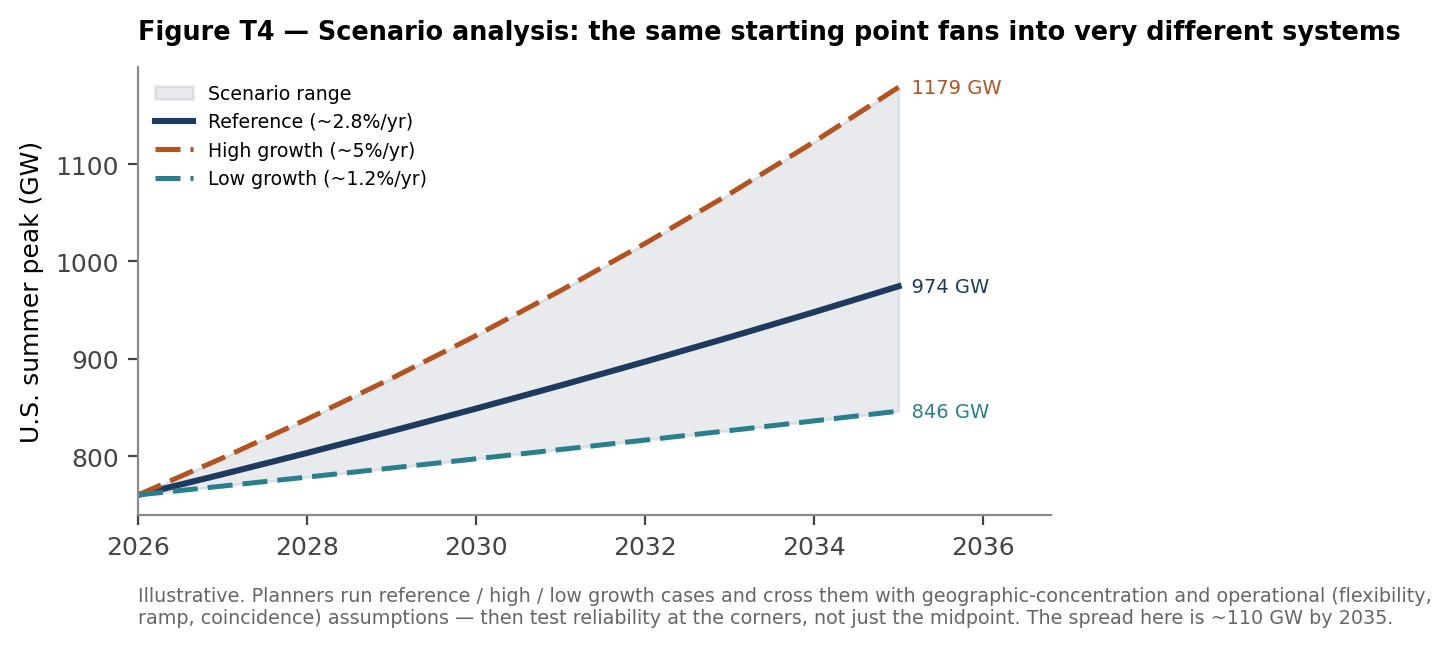
Figure T4 — Scenario analysis in one picture: a single starting point fans into materially different systems depending on assumptions about load growth, resource cost and policy. The spread matters because a plan optimised for the central case frequently proves the worst under both tails. The implication for a planner is that scenarios are not a way of improving a forecast but a way of identifying which commitments are robust across futures and which depend on one arriving — so reliability should be tested at the corners of this space, not only along the reference line.
The purpose is not to predict which scenario occurs but to find robust decisions and no-regret moves — upgrades and reforms that pay off across the range — and to identify the scenarios in which the system fails, so those can be monitored and hedged. Flexible-load service (Section 6) attracts precisely because it comes close to no-regret: it helps in the high-growth case and costs little in the low. NERC's May 2026 guideline pushes exactly this way, asking for resource-adequacy studies evaluated across many weather, load, and outage combinations on a network-aware footprint rather than against a single deterministic peak.
T.8 Reliability assessment: the metrics a study must satisfy (supports Sections 4 and 2)#
Why this section exists, and what the criteria do. The metrics here are the pass-fail conditions that convert a simulation into a decision. A stability study produces voltage and frequency traces; the criteria in this section state which traces are acceptable, and they supply the operative content of any performance obligation. This matters for Section 4 in a specific way: a ride-through requirement is nothing more than a stated voltage-duration envelope that equipment must remain connected through, so the argument about whether such requirements are reasonable is an argument about where to draw the boundary of that envelope. The contingency categories below serve the same function for the network, defining which events a planner must design against and which are treated as beyond the standard.
Reliability assessment is where all the preceding analysis is scored: given a future load condition, does the system stay within its steady-state and dynamic limits under the required contingencies? The checks fall into two families. Steady-state assessment confirms that, in the base case and under each contingency, no element exceeds its thermal rating and every bus voltage stays within limits (typically 0.95–1.05 per unit). Dynamic assessment exposes large loads. It evaluates the system's time-domain response to disturbances against three families of metric. Transient, or angular, stability asks whether machines stay in synchronism. Frequency response covers the rate of change of frequency (RoCoF) immediately after a loss, the frequency nadir, and the settling value; all three worsen as inverter-interfaced load displaces inertia. Post-fault voltage recovery covers fault-induced delayed voltage recovery (FIDVR), where stalled motors or tripping loads hold voltage down after the fault clears. Small-signal (oscillatory) stability draws increasing concern because synchronized AI workloads can act as a forcing function that excites weakly damped inter-area modes (T.2).
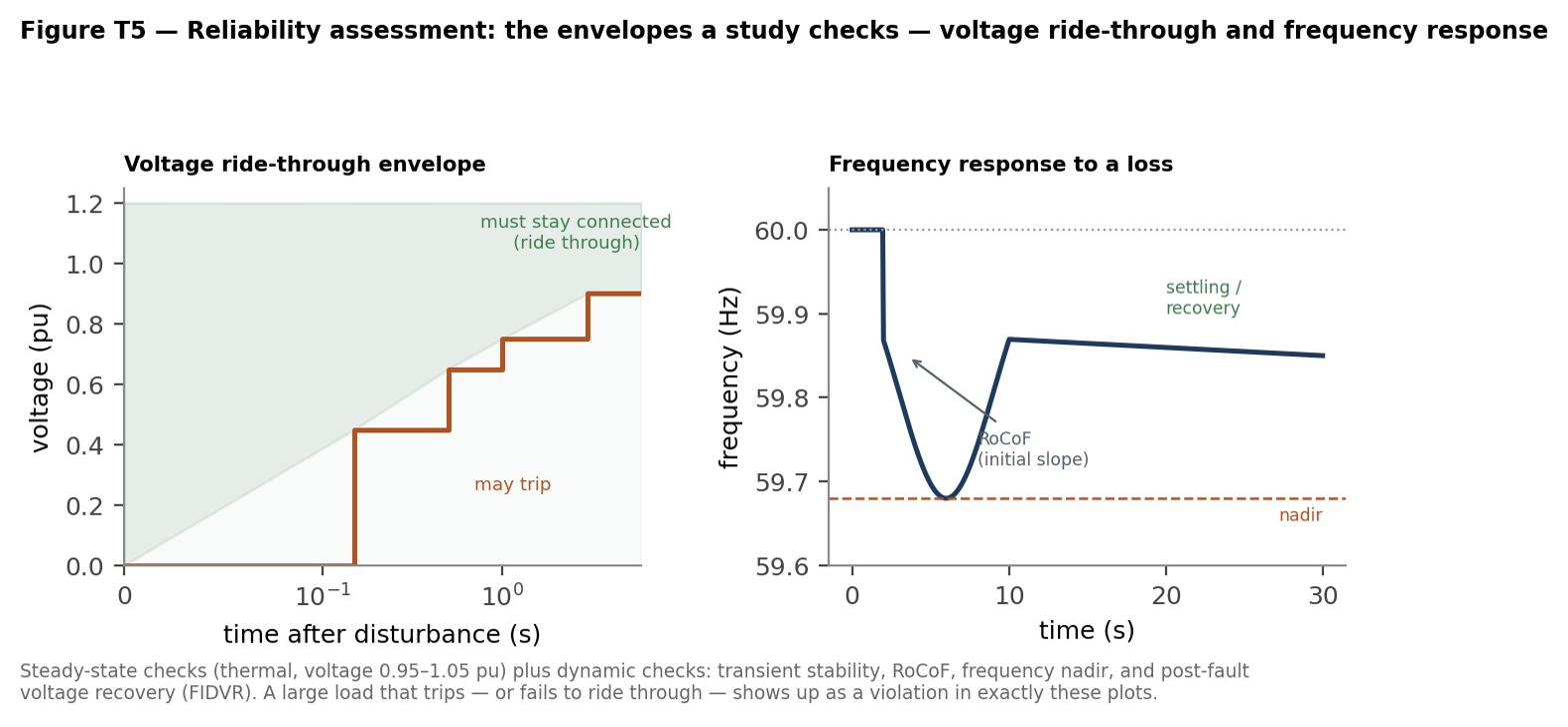
Figure T5 — The two envelopes a reliability study checks. Left: the voltage ride-through envelope a large load must stay connected through. Right: the frequency response to a sudden loss, with the RoCoF, nadir, and recovery a study evaluates.
Protection coordination. The envelopes above describe when a load should stay connected; protection settings decide when it will actually trip, and the two do not coincide. A large computational load sits behind layered protection — utility relays at the point of interconnection, the facility’s own main and feeder breakers, and the fast electronic protection inside every UPS and power supply — which must be coordinated so that a fault clears at the smallest affected zone rather than disconnecting the whole campus. Three settings dominate the recent ride-through record. Undervoltage and under-frequency trip thresholds, often left at a vendor default, can fire well inside the envelope that PRC-024 and the newer PRC-029 require loads to hold. Anti-islanding protection, meant to disconnect on-site generation when the grid is lost, can misread a deep transmission voltage sag as an island and trip. And breaker-and-relay timing graded for a conventional load — a downstream device clearing before an upstream one — can invert when converter front ends inject or withhold fault current in ways the coordination study never assumed. The consequence is that ride-through is a protection problem as much as a control problem: a load can carry a compliant controller and still trip on a mis-set relay, and a coordination study built on static, motor-dominated load will not catch it (Technical Annex T.3).
The contingency set is defined by TPL-001, which enumerates event categories from the everyday (P0, no contingency; P1, loss of a single element) through more severe multiple-element events (up to P7). For most categories the standard permits no non-consequential load loss — which explains why an uncommanded large-load trip during a normally-cleared fault (Section 4) raises a reliability-standard problem rather than an inconvenience: the criteria say that load loss should not occur. The through-line of this annex is that a reliability assessment is only as trustworthy as the load model feeding it (T.4), the contingencies it considers (T.3), and the scenarios it spans (T.7). Get those right and the metrics in this figure tell you whether the future grid holds; get them wrong — as a static load model does — and the study will certify a system that will not.
T.9 Distribution-system impacts: the layer the bulk-power debate skips (supports the Primer and Section 3)#
Why this section exists. The whole report is written about the bulk power system because that is where gigawatt campuses connect, and this section covers the consequence of that focus. Two effects run in opposite directions. A facility connecting at transmission voltage bypasses the distribution system, contributing little to its cost while still influencing the wholesale prices that distribution customers pay — a cost-allocation question rather than an engineering one. Meanwhile the faster-growing population of smaller sites lands directly on feeders designed for diverse residential and commercial demand, where the planning tools, the protection settings and the hosting-capacity assumptions were all calibrated on a load that behaved differently. The bulk-system reforms in Sections 1 through 6 reach none of these smaller facilities.
Almost everything in this report concerns the bulk power system — transmission, wholesale markets, and systemwide reliability. That focus holds for the gigawatt campuses that dominate the headlines, because a load that large connects directly at transmission or sub-transmission voltage and largely bypasses the distribution system altogether. But that very fact creates two distinct distribution-level stories worth naming.
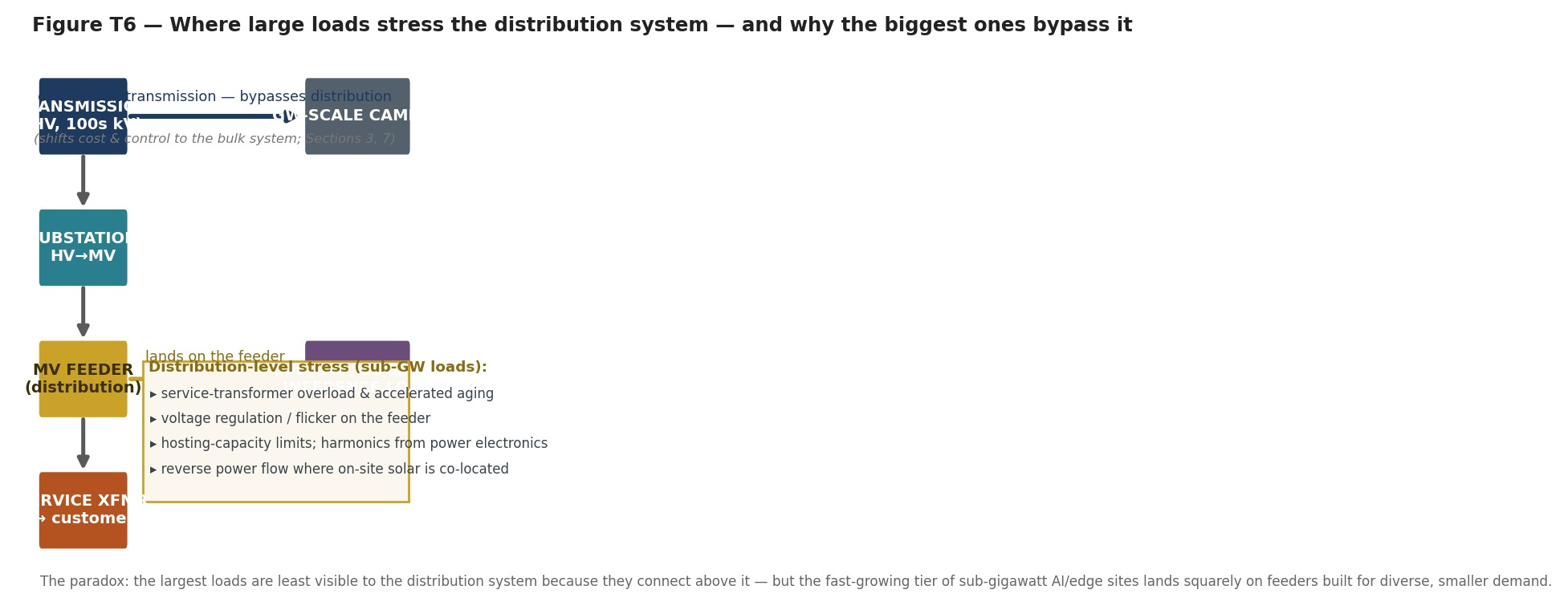
Figure T6 — The largest loads remain least visible to the distribution system because they connect above it; the fast-growing tier of sub-gigawatt AI, edge, and inference sites lands squarely on feeders built for smaller, diverse demand.
The first story concerns what the bypass itself does. When a hyperscale campus interconnects at transmission, it contributes little to distribution-system cost yet still shapes the wholesale prices and capacity charges that flow through to distribution customers' bills — which is part of why the cost-allocation fight in Section 3 plays out at the wholesale and state-tariff level rather than in distribution rate cases. The load is physically absent from the feeder but financially present on the bill. The second story is the fast-growing tier that does not bypass distribution: sub-gigawatt colocation, “edge” facilities, and AI-inference sites in the tens-to-low-hundreds of megawatts, which increasingly land on medium-voltage feeders and distribution substations that were planned for diverse, smaller commercial demand. There the classic distribution problems reappear at new intensity. Service transformers and feeders overload and age faster. Voltage regulation and flicker suffer as large, fast-varying loads swing; hosting-capacity limits and harmonic distortion injected by the same power-electronic front ends discussed in T.1; and, where on-site solar or storage is co-located, reverse power flow that distribution protection was never designed for. Utilities are responding with distribution-level hosting-capacity analysis, interconnection screens, and — as at the transmission level — flexible or curtailable connection terms. The distribution–transmission coordination gap poses the subtler risk: a load small enough to count as a distribution matter can still, in aggregate with its neighbors, present a transmission-scale contingency, and the two planning worlds do not always talk to each other. This is the same firm-versus-flexible and modeling discipline as the rest of the annex, applied one voltage level down.
For a nonspecialist the useful correction is that a gigawatt of new load is not automatically a transmission problem. Which element binds first depends on where and how the load connects. A campus that interconnects at extra-high voltage may never touch a distribution feeder, while a cluster of inference sites at medium voltage can exhaust a substation transformer, a feeder breaker’s interrupting rating, or the station bus long before any transmission limit appears. The screening order runs from the device outward — transformer and breaker ratings, then feeder thermal and voltage-regulation limits, then the substation bus — and only then to the bulk-power constraints the rest of this report treats. The debate defaults to transmission because that is where the largest campuses connect; the fast-growing tier does not, and its first constraint usually sits one voltage level down.
T.10 Planning paradigms and tools: deterministic vs. probabilistic, and how they fit together (supports Sections 1, 2, and 9)#
Why this section exists. The preceding sections describe tools that answer different questions in incompatible languages, and a reader encountering them separately can reasonably conclude they conflict. They do not. A deterministic study asks whether a specified condition is survivable and returns yes or no; a probabilistic assessment asks how often adverse conditions arise and returns a frequency. Neither substitutes for the other: a probabilistic result cannot tell an engineer whether a particular bus stays within its voltage band, and a deterministic study cannot tell a planner whether the condition it examined is likely enough to warrant the cost of preventing it. The practical relationship is sequential — probabilistic methods identify which conditions merit deterministic examination, and deterministic studies establish what must be built if those conditions occur.
The report introduces forecasting (T.5), adequacy (T.6), and scenarios (T.7) separately; this part gives the nonspecialist the single frame that connects them. Grid planning has been undergoing a slow migration from a deterministic to a probabilistic paradigm, and the large-load problem is accelerating it. Deterministic planning tests the system against a fixed set of defined conditions — a forecast peak, a specified list of contingencies (the N-1/N-1-1 events of TPL-001), a design-day weather assumption — and asks whether it holds in each. It stays transparent and auditable, exactly what a reliability standard needs — the reason the contingency framework in T.3 and T.8 runs deterministic at its core. It says nothing about how likely each condition runs, and combinations no single scenario captured can blindside it. Probabilistic planning instead runs the system across a distribution of conditions — many weather years, forced-outage draws, and load realizations — and reports outcomes as likelihoods: the loss-of-load expectation, hours, and unserved-energy metrics of T.6 are inherently probabilistic. The two are complements, not rivals: deterministic analysis sets the pass/fail reliability floor, probabilistic analysis sizes the margin and prices the risk. Large, uncertain, flexible loads push planners toward the probabilistic end because a single deterministic peak cannot represent a load that might materialize or might curtail. Three tool families do the work, each answering a different question:
- Power-flow and stability tools (deterministic). Answer “does the network hold under this condition?” — the steady-state, short-circuit, transient, and EMT studies of T.3–T.4. Used for interconnection and reliability compliance.
- Production cost models (PCM). Chronological simulations of the whole market — hour-by-hour (or finer) unit commitment and economic dispatch across a year — answering “what does the system cost to run, where does congestion bind, and what are the emissions and prices?” Planners use such tools to test whether a large load raises congestion or curtails renewables, and how flexible load changes dispatch. They sit between deterministic and probabilistic: one PCM run stays deterministic, but planners sweep many to explore the range.
- Resource-adequacy models (probabilistic). Monte Carlo simulations (the ProbA of T.6) that answer “is there enough accredited capacity, and how often will we fall short?” — producing LOLE/LOLH/EUE and the ELCC accreditations that decide whether a flexible load counts as a resource. A well-run planning process uses all three and the scenario discipline of T.7 on top: deterministic studies to certify reliability, production cost modeling to understand economics and congestion, and probabilistic adequacy modeling to size reserves — each run across a range of futures rather than a single forecast. The large-load era's methodological lesson is simply that the deterministic single-number habit is no longer sufficient on its own; the uncertainty is now too large to leave unquantified.
| Horizon | The decision it answers | Tool or model | Where |
|---|---|---|---|
| Seconds to minutes | Hold frequency and voltage instant to instant, and ride through disturbances | Automatic generation control; operator action | T.11 |
| Minutes to an hour | The cheapest safe dispatch of the units already committed | Security-constrained economic dispatch | T.11 |
| Hours to days | Which units to start, stop, and hold in reserve | Unit commitment; production-cost models | T.10 |
| One to five years | Whether accredited capacity meets the reliability standard | Resource-adequacy (probabilistic) assessment | T.6 |
| Five to twenty years | What to build and retire, and which lines to add | Integrated resource plans; transmission planning | T.5, T.7 |
Table T10A — The same grid, planned on five clocks. Each horizon carries its own tool and its own question; much of the large-load debate confuses the two — answering a years-scale adequacy question with a seconds-scale operations instinct, or the reverse. The tools complement rather than compete, and the annex sections in the final column treat each in turn.
T.11 Operational impacts: what large loads do to the control room (supports Sections 4 and 6)#
Why this section exists. The preceding annex sections describe how large loads are studied, forecast, modelled and planned for. None describes what happens once the load is energised and an operator has to run the system around it. The distinction matters because the planning tools work in hours and years while the control room works in seconds and minutes, and the three characteristics that make computational load hard to plan for — magnitude, speed, and opacity — bear on operations more immediately. Four places where that shows up are sketched below. This is a map of where the operational discussion is heading in NERC and ISO forums rather than a settled account; the standards work described in Section 4 will determine most of it.
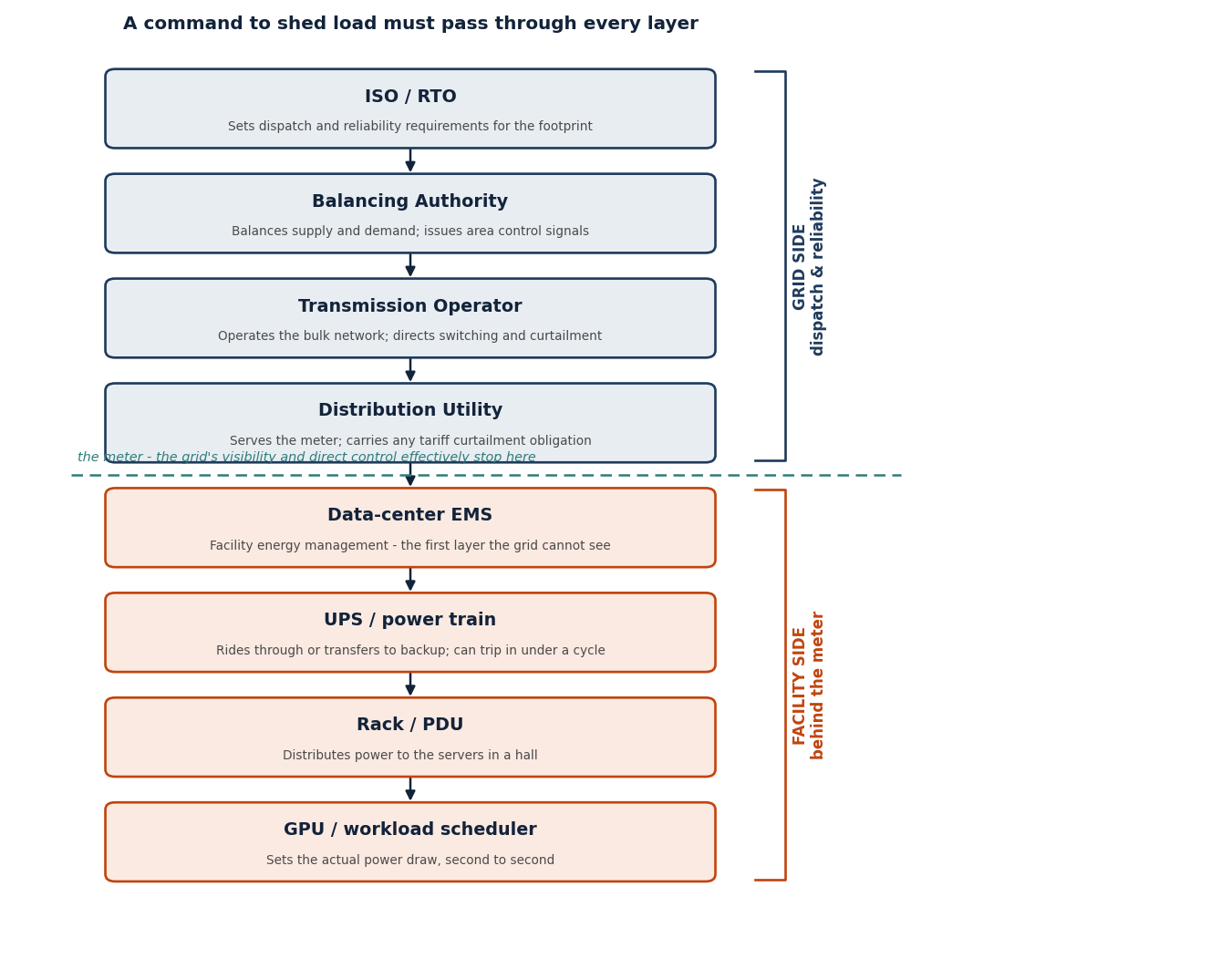
Figure T8 — The control hierarchy: who actually commands a large load. A curtailment instruction must pass through four grid-side layers and four inside the facility. The grid’s visibility and direct control effectively end at the meter; below it, the load’s second-to-second draw is set by equipment and a workload scheduler the operator cannot see — which is why a load’s flexibility is usable only when the settings below the meter are configured to honour it.
- Situational awareness and the EMS. An operator acts on what the energy management system shows, and computational load ranks as the least visible large object on the system: it sits behind a customer meter, its internal state is not telemetered, and its next move is set by a workload scheduler the operator cannot see. State estimation and contingency analysis run against a model carrying the load as a static MW value, so the telemetry and registration requirements of Section 4 pose an operations problem as much as a planning one. Until the control room can see a campus's ramp capability and its ride-through settings, the three items below are being managed from an incomplete picture.
- Ramping and dispatch. Economic dispatch solves every five minutes against a load forecast built from historically smooth behaviour. Training workloads step between power states in seconds and can move tens or hundreds of megawatts inside a single dispatch interval, so the ramp reaches the market as forecast error and is covered by the fastest and most expensive resources on the stack. The mitigation is the flexibility of Section 6 read from the other end: a load that shapes its own ramp serves the dispatch better than one that must be chased.
- Regulation and AGC. Automatic generation control corrects the second-to-second imbalance that dispatch leaves behind, acting on area control error — the combined measure of frequency deviation and net interchange error that records whether a balancing authority is carrying its own load. Regulating reserve is procured against the expected variability of net load. Where a campus swings faster than the regulating fleet responds, ACE degrades and the balancing authority's control performance measures (BAL-001, BAL-003) move in the wrong direction — a compliance exposure before it becomes a reliability one.
- Reserve deployment and the loss-of-load contingency. Contingency reserve is sized against the largest single contingency, historically a generator or a tie line. A gigawatt campus that trips off — or rides through and then returns — presents a contingency of comparable size at the other end of the balance, one that can repeat within minutes rather than once a day. The operational question is therefore not only how much reserve is carried, but whether reserve deployed for a load-side event can be restored before the next one, which is the control-room form of the ride-through argument in Section 4.
Sources: NERC reliability standards BAL-001 and BAL-003; the large-load registration and modelling work of Project 2026-01 and RD26-7-000; NERC and ISO workshop material on data-center operating characteristics. This section is an engineering synthesis rather than a report of filed positions.
T.12 Classifying flexibility: the Flex MOSAIC framework (supports Sections 1 and 6)#
Why this section exists. Section 6 argues that the obstacle to flexible service is machinery rather than physics — that no one has built the contractual and operational terms. A classification is the first of those terms, because a utility and a customer cannot contract over a capability they describe differently. This part sets out the framework the industry settled on in March 2026, at the level of detail a connection study would need. The argument about what it means for who writes the rules is in Section 7; the argument about whether the flexibility is real is in Section 6.
EPRI released Flex MOSAIC at CERAWeek on March 23, 2026, developed through the DCFlex initiative with more than sixty-five utilities, system operators, regulators, hyperscalers and technology providers. It is voluntary, and it is technology-neutral by construction: it describes what a load can do rather than the equipment that does it, so a facility using workload scheduling and one using on-site storage can make the same commitment in the same words.
The six performance characteristics. A load's flexibility is described by notification time, duration, frequency of use, depth of load adjustment, ramp behaviour, and availability. Five of the six are the terms Section 6's assessment asks a curtailment product to state, which is why the framework matters more than a classification usually would.
The five classes. The characteristics group into five lettered classes, each matched to a system need rather than to a technology. Class A supports the system through infrequent extreme stress. Class B manages daily or weekly demand peaks. Class C meets sustained energy shortages. Class D responds to sudden swings in supply or demand. Class E provides frequency stabilisation. EPRI's own reading is that D and E unlock the most system value, because they address local thermal overloads and voltage depressions — which is the same point Section 3 makes about deliverability rather than supply being the binding constraint. Class descriptions reported from trade coverage of the launch; the framework's own class table has not been read against this text.
What delivers it. EPRI groups the means into three pillars: managed workloads, reduced energy consumption within the AI plant itself, and back-up power. The second is the layer Annex T.1 describes — ramp limits, power floors and rack-level storage — which places the equipment designs of 2025–26 inside the classification rather than beside it. The third raises a question the framework does not settle: back-up generation dispatched for grid benefit is a resource, with the permitting and emissions consequences Section 5 sets out, and calling it flexibility does not make it something else.
What the framework is for. Its stated purpose is speed to power. A common vocabulary lets flexibility be counted during the connection study rather than modelled case by case under conservative assumptions, which is a route through the queue that does not require a tariff (Section 1). Five guiding principles govern it: non-discrimination, transparency, completeness, standardisation, and adoptability. The first two are regulatory concepts appearing in a voluntary industry document, which is the tell that the framework anticipates being written into tariffs — and the reason Section 7 treats it as private ordering ahead of public rulemaking rather than as a technical standard.